| The followings are examples applications using models developed from the Discrete Element Method (DEM) or the coupling method with the Thermal fluid flow analysis. |
| Particle-fluid coupling scheme considering the pore water pressure. |
 |
1. Introduction
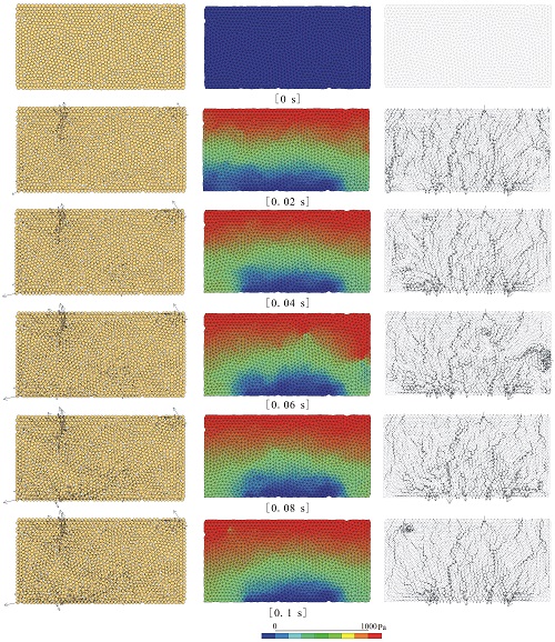
Figure 1 shows a fluid grid (fluid cell) created inside the group of particles using this scheme for two- or three-dimensions. The whole domain composed by the group of particles, whose shape is a spherical (three-dimension) or a circular shape (two-dimension), is divided by a tetrahedron shape (three-dimension) or a triangular shape (two-dimension) fluid grid. Each fluid grid is defined by adjoining the volumetric center of the nearest particles (four particles: three-dimension, three particles: two dimension). Fluid grid expresses as a fluid reservoir that exists in gaps (void spaces) between particles. The porosity and fluid pressure; pore water pressure are defined by their volumetric center, and each fluid grid conserves the continuity. Fluid flows through boundaries between each neighboring fluid grids due to the pressure difference. The fluid pressure changes for each fluid grid due to the relative motion of particles and fluid flow through the boundary. A body force, which is calculated by multiplying the fluid pressure by area occupied by fluid, is applied to the particles. Since the contact on the Discrete Element Method uses soft contact approach, the particles are treated as rigid body which allows an overlap between particles. Accordingly, the volume calculation of void spaces is also considered to have overlaps between particles. Figure 2 shows a numerical result on underground flow using this scheme. The difference in void spaces enables to simulate localization of flow.
|
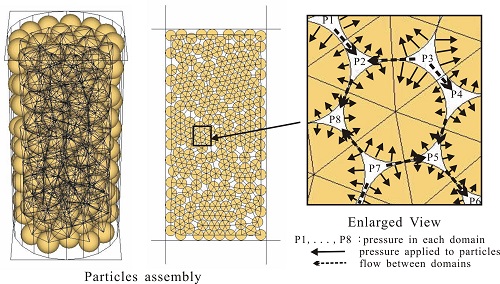 |
| Figure1 Fluid cells created on void spaces in particle assembly. |
| Figure 2 General View: transient particle displacement (left), water pressure (middle)
and apparent water pressure (right).
|
2. Simulation of debris flow
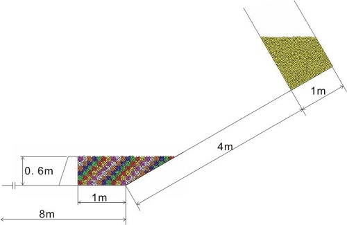
Figure 3 shows the numerical model. This numerical model is made by connecting horizontal and inclined waterway having width of 0.6m; horizontal waterway of 8m and inclined waterway of 4m with 30 degree slope, and adding a holding section with water sealed gate provided with debris flow particles on the upper section. These dimensions mimic experimental set-up. The model is created by using the two dimensional wall element (a line element) of each horizontal and inclined waterway. The dam model is made by adding line elements as well. The particle holding section and the dam section are each placed with particles modeled as flowing and accumulated debris. For the particles to be placed on the dam section, different colors are used for each 10 cm x 10 cm in order to make movements of particles flowing downwards (particles in debris flow) clear. |
| Figure3 Numerical model, initial state. |
Figure 4 shows the movement of debris flow and accumulated particles during its saturated state for each 0.5 seconds, starting from 0.5 seconds after the point of deleting of the wall corresponding to the gate, up to 8 seconds. The calculated result in the case of saturated condition shows a significant rise in pore water pressure when the debris particles collided with accumulated particles in the dam section, and were able to notice the particles that accumulated high went over the dam and flowed downwards. Moreover, it takes a long time for the system to become stable after the debris particles flowed down and collided with the volume particles in the dam section.
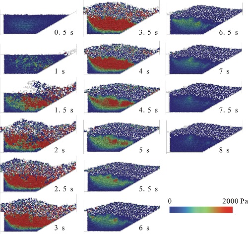
Figure 5 shows pore water pressure between inside particle and debris flow particles on the upper part of flowing dam of saturated condition for each 0.5 seconds, starting from 0.5 seconds after the point of deleting the wall corresponding to the gate, up to 8 seconds. After one second the debris flow particles starts colliding with accumulated particles, and the pore water pressure starts becoming greater in front of upper flow of dam, and its effects starts spreading to the whole upper section. With the after effects of the collision of debris flow particles making the debris flow particles to add up to the upper part of volume particles, almost all pore water pressure inside accumulated particles of dam section increases, with exception of the lower section. This effect lasts even after the movement of particles ceased almost completely and accumulated condition became stable, its water pressure subsides little by little and by 8 seconds after the pressure returns to its normal condition almost completely.
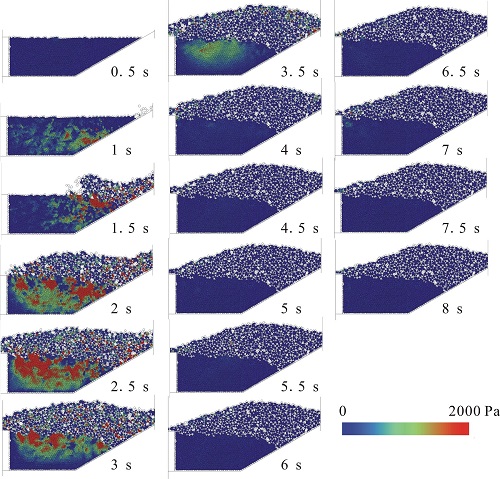
Figure 6 shows a calculated result in the case of multiplying the permeability of figure 5 by 10. When comparing with the result in Figure 5, the level of excess pore water pressure inside particles rests low, and the time for the pressure to increase and then to subside is relatively short. After 4 seconds from deleting the wall on the gate, pore water pressure that rised up went back to its initial level. Also, the rise of debris flow particles during collision is insignificant. Since effective stress of debris flow particles decreases when the excess pore water pressure occur, and the resistance becomes weak, it triggers the fluidization of debris sand and the moving fast in long distance, and the particles that overflow seems to increase.
|
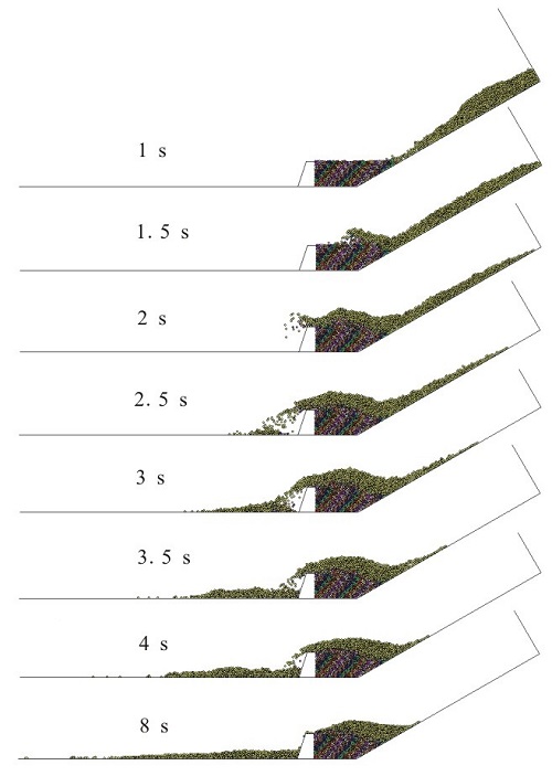 |
| Figure4 Movement of debris flow and accumulated particles,
saturated condition, 1-8 seconds.
|
| Figure 5 Changes in pore water pressure on upper dam section and inside accumulated particles, permeability 1.2x10⁻²cm/s,0.5-8 sec. |
| Figure 6 Changes in pore water pressure on upper dam section and inside accumulated particles, permeability 1.2x10⁻¹cm/s,0.5-8 sec. |
3. Simulation of liquefaction
Figure 7 shows a numerical model; (a). particle assembly, (b). fluid cells. Particles are created with a height of 0.4m inside a rectangular wall with width of 0.8m. The particles were made to have a cylindrical shape with depth of 0.2m, the average particle diameter of 20mm having ±20% particle size distribution. This model was made with two conditions (loose state: initial porosity 0.20, two-dimension, tight state: initial porosity 0.16, two-dimension). After preparing initial state, the conditions equaling a centrifuge model experiments are applied to the numerical model and pore water pressure, effective stress, and particle acceleration are recorded. The applying conditions are a 200gal for practical material, and 20 waves of 1Hz sinusoidal wave are added. The analytical time is 5.0 or 25.0 seconds. |
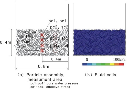 |
Figure 8 shows evolution of excess pore water pressure in the case of 0.20 initial porosity. In this case, when acceleration begins, changes of pore water pressure can be seen for each parts inside the particle assembly, and the pore water pressure gradually becomes greater. Change of pore water pressure in the lower part is greater compared to the upper layer. Moreover, pore water pressure is not distributed equally in horizontal direction, but have differences locally.
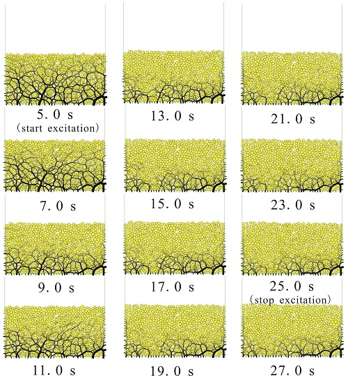
Figure 9 shows evolutions of contact force. In the figure, the contact forces between particles shown in black lines have different thickness according to its strength. In this case, the contact force applying to the weight of particles underwater is shown to increase as the depth of layer of particles becomes lower at first, but as the acceleration is put into place, contact force between particles decreases gradually from the upper layer of particles. Furthermore, when comparing in Figure 8, for areas with strong contact force in the lower section of particle layer , the excess pore water pressure becomes stronger due to acceleration, and progression of liquefaction and decrease of contact force can be seen as well.
|
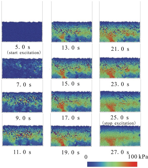 |
| Figure8 General view: transient of pore water pressure, initial porosity 0.20. |
| Figure9 General view: transient of contact force, initial porosity 0.20. |
References
1). Shimizu, Y., Microscopic Numerical Model of Fluid Flow in Granular Material, Geotechnique, vol.61, no.10, pp.887-896, (2011)
2). Shimizu, Y. et al., A numerical simulation on centrifuge liquefaction model using microscopic fluid coupling scheme with Discrete Element Method, Proc. of 7th European Conf. on Numerical Methods in Geotechnical Eng., Trondheim, Norway, pp.201-206, (2010).
3). Shimizu, Y. and Inagawa, Y., Numerical Study on Liquefaction Using Discrete Element Method with Microscopic Fluid Coupling Scheme, JSCE/C, vol.66, no.4, pp.800-813, (2010)
4). Shimizu, Y. OCHIAI, H. and OKADA, Y., DEM Simulations of Debris Flow Using Microscopic Fluid Coupling Scheme, JSCE/C, vol.65, no.3, pp.633-643, (2009)
|
|
|
|